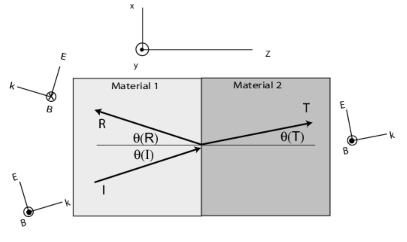
EM propagation at oblique incidence to an interface between dissimilar dielectric media

From EM-class we know $$ \begin{align} E_I \cos \theta_I + E_R \cos \theta_R &= E_T \cos \theta_T, \\ \epsilon_1 (-E_I \sin \theta_I + E_R \sin \theta_R) &= -\epsilon_2 E_T \sin \theta_T, \end{align} $$ this can be simplified to $$ \begin{align} 1 + r &= \alpha t, \\ 1 - r &= \beta t, \end{align} $$ where \( \alpha \) and \( \beta \) are defined as $$ \begin{align} \alpha &\equiv \frac{ \cos \theta_T }{ \cos \theta_I}, \\ \beta &\equiv \frac{ n_1 }{ n_2 } \frac{ \epsilon_2 }{ \epsilon_1 }. \end{align} $$ From above we can derive $$ \begin{align} t &= \frac{ 2 }{ \alpha + \beta }, \\ r &= \frac{ \alpha - \beta }{\alpha + \beta }. \end{align} $$ We can even delve further that $$ \begin{align} \alpha &= \frac{ \sqrt{1 - \big( \frac{ n_1 }{ n_2 } \big)^2 \sin^2 \theta_I} }{ \cos \theta_I }, \\ \beta &= \tan \theta_B, \end{align} $$ where \( \theta_B \) is called Brewster angle.

Here we assume the following plane-wave is only p-polarized, that is, \( \tilde{\mathbf{ E }} \) only has \( \hat{\mathbf{ x }} \) and \( \hat{\mathbf{ z }} \) components. The Poynting vector is $$ \mathbf{ S } = \frac{ 1 }{ \mu_0 } \mathbf{ E } \times \mathbf{ B }, $$ with unit \( \frac{ \text{W} }{ \text{m}^2 } \), here \( \mathbf{ E } = \Re{(\tilde{\mathbf{ E }})} \), \( \mathbf{ B } = \Re{( \tilde{\mathbf{ B }} )} \). Or it can be expressed as complex form: $$ \begin{equation} \begin{split} \mathbf{ S } &= \frac{ 1 }{ \mu_0 } \mathbf{ E } \times \mathbf{ B } \\ &= \frac{ 1 }{ \mu_0 } \Re{(\tilde{E})} \Re{( \tilde{B} )} \hat{\mathbf{ k }} \\ &= \frac{ 1 }{ 4\mu_0 } (\tilde{E}\tilde{B} + \tilde{E}\tilde{B}^\ast + \tilde{E}^\ast\tilde{B} + \tilde{E}^\ast\tilde{B}^\ast)\hat{\mathbf{ k }} \\ &= \frac{ 1 }{ 2\mu_0 } \Big[ \Re{ (\tilde{E} \tilde{B}) } + \Re{ (\tilde{E} \tilde{B}^\ast) } \Big]\hat{\mathbf{ k }}, \end{split} \end{equation} $$ where \( \tilde{E} = \tilde{E}_0 e^{i (\mathbf{ k } \cdot \mathbf{ r } - \omega t)} \), \( \tilde{B} = \tilde{B}_0 e^{i (\mathbf{ k } \cdot \mathbf{ r } - \omega t)} \).

The time-averaged intensity is $$ I = \langle S \rangle = \frac{ \omega }{ 2\pi } \int_{0}^{2\pi/\omega} S(t) \, dt = \frac{ 1 }{ 2 } \sqrt{\frac{ \varepsilon_0 \varepsilon_r }{ \mu_0 }} E_0^2 = \frac{ 1 }{ 2 } c \varepsilon_0 n E_0^2, $$ where \( E_0 = \sqrt{\tilde{E} \tilde{E}^\ast} \).

In the simulation below, for instantaneous intensity, I plot the norm of the Poynting vector at every spatial point; for time-averaged intensity, I plot \( \langle S \rangle \) at every point; for E-field, I plot the magnitude of the real-part of E-field.

Note: This simulation does not consider total internal reflection, so results above critical angle may be inaccurate.

Questions

1. Identify Brewster angle on either left or right panel. What is the relation between \( \theta_B \) and \( \theta_T \) when a light is incident at this angle?
2. Observe the amplitude of reflective and transmitted light. How do they change when \( \theta_I \), \( n_1 \), and \( n_2 \) change? How do reflected and transmitted intensity change?